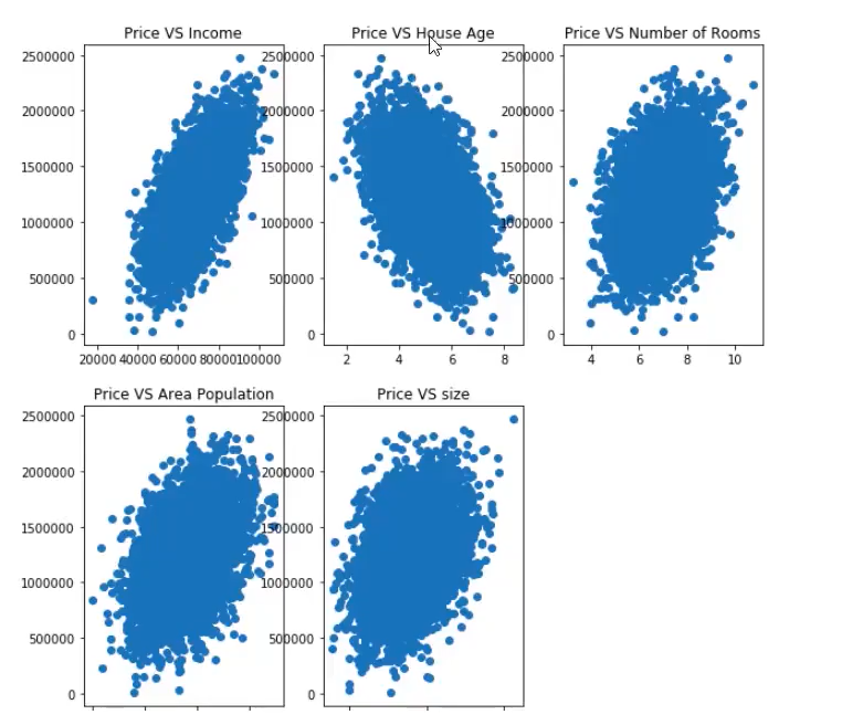
# visualizing data # 内嵌绘图,可省略 plt.show() 这一步 %matplotlib inline from matplotlib import pyplot as plt fig = plt.figure(figsize=(10,10)) fig1 = plt.subplot(231) # 两行三列第一个图 plt.scatter(data.loc[:,'Avg. Area Income'],data.loc[:,'Price']) plt.title('Price VS Income')
fig2 = plt.subplot(232) # 两行三列第二个图 plt.scatter(data.loc[:,'Avg. Area House Age'],data.loc[:,'Price']) plt.title('Price VS House Age')
fig3 = plt.subplot(233) # 两行三列第三个图 plt.scatter(data.loc[:,'Avg. Area Number of Rooms'],data.loc[:,'Price']) plt.title('Price VS Number of Rooms')
fig4 = plt.subplot(234) # 两行三列第四个图 plt.scatter(data.loc[:,'Area Population'],data.loc[:,'Price']) plt.title('Price VS Area Population')
fig5 = plt.subplot(235) # 两行三列第五个图 plt.scatter(data.loc[:,'size'],data.loc[:,'Price']) plt.title('Price VS size')
plt.show() # 可以省略
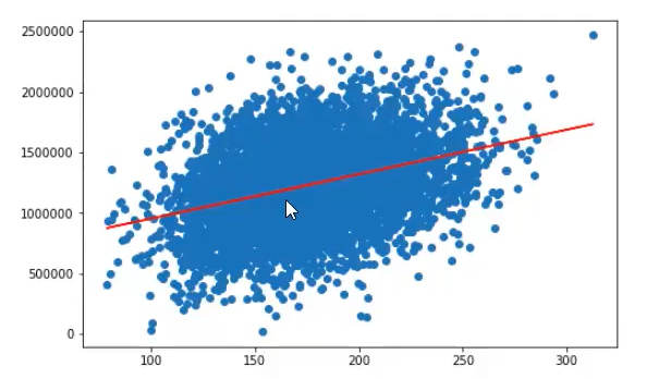
3. 建立单因子模型(面积)
(1)定义 X、Y
X:影响因素;Y:结果值
1 2 3 4
# define x and y X = data.loc[:,'size'] y = data.loc[:,'Price'] y.head()
(2)建立回归模型
1 2 3 4 5 6 7 8
# set up the linear regression model from sklearn.linear_model import LinearRegression LR1 = LinearRegression() # reshape data X = np.array(X).reshape(-1,1) print(X.shape) # train the model LR1.fit(X,y)
(3)模型预测
1 2 3
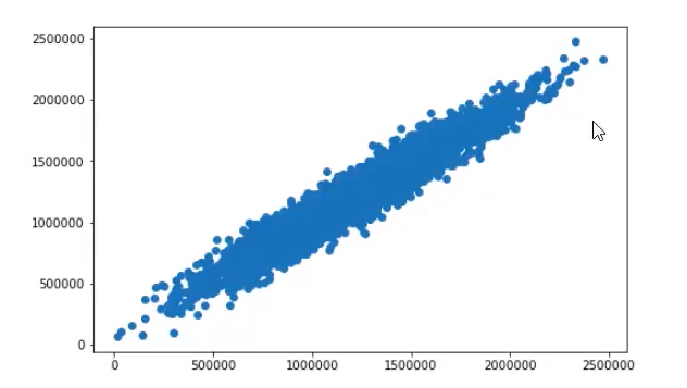
# calulate the price vs size y_predict_1 = LR1.predict(X) print(y_predict_1)
(4)模型评估
1 2 3 4 5
# evaluate the model
from sklearn.metrics import mean_squared_error,r2_score
mean_squared_error_1 = mean_squared_error(y,y_predict_1)
r2_score_1 = r2_score(y,y_predict_1)
print(mean_squared_error_1,r2_score_1)